[Fujimoto, Saito]

The issue of the low DC output from the RFPD reported previously (klog:37436) was resolved by reconnecting the cable. Next, an HWP was installed in front of the BS for the sub-laser, and the polarization was set to S-polarization. When the beat signal was observed, the peak was split into two. By rotating either the HWP in front of the BS or the polarizer in front of the RFPD, the relative amplitudes of the two peaks could be changed. Therefore, it appears that the P-polarization peak is also being observed simultaneously, and this is likely caused by birefringence in ITMY. The results of determining the SRY length from the beat signal data acquired while maximizing each of the two peaks will be posted later.
 

• First, to investigate the reason for the low DC output from the RFPD reported previously (klog:37436), we monitored the DC output of the RFPD with an oscilloscope and found it to be approximately 8 V. Since there was no problem with the signal amplitude and the fluctuations were not significant, we reconnected the RFPD to CDS, and the DC output was approximately 12500 counts, corresponding to approximately 7.6 V. Therefore, the connection may not have been good in the previous measurement (klog:37436).
   
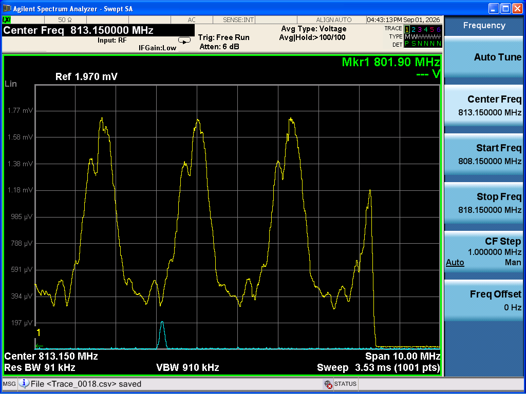
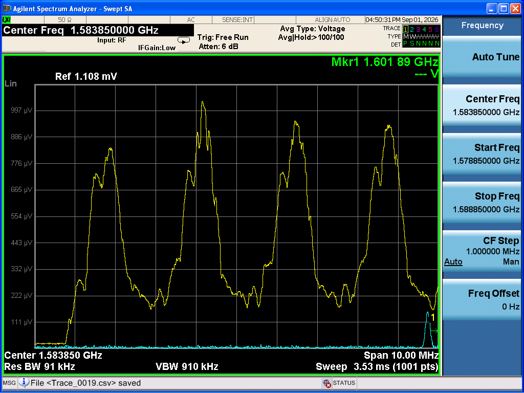
• Next, an HWP was installed in front of the BS for the sub-laser (Photo 1), and the polarization was set to S-polarization using a PBS. The main laser was then turned off, and the sub-laser was aligned to SRY. When we observed the beat signal at -1.6 GHz, the peak was split into two (Photo 2). We then rotated the polarizer in front of the RFPD. This allowed us to decrease the amplitude of one peak while increasing that of the other. Similarly, rotating the HWP installed in front of the BS also allowed us to change the relative amplitudes of the two peaks. Therefore, although the sub-laser was initially set to S-polarization, the measured beat signal contains a P-polarization component. This is likely due to birefringence in ITMY.
   

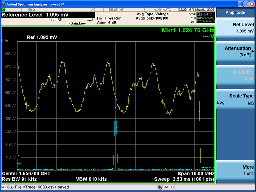
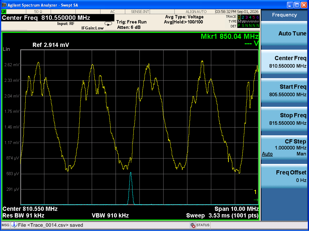
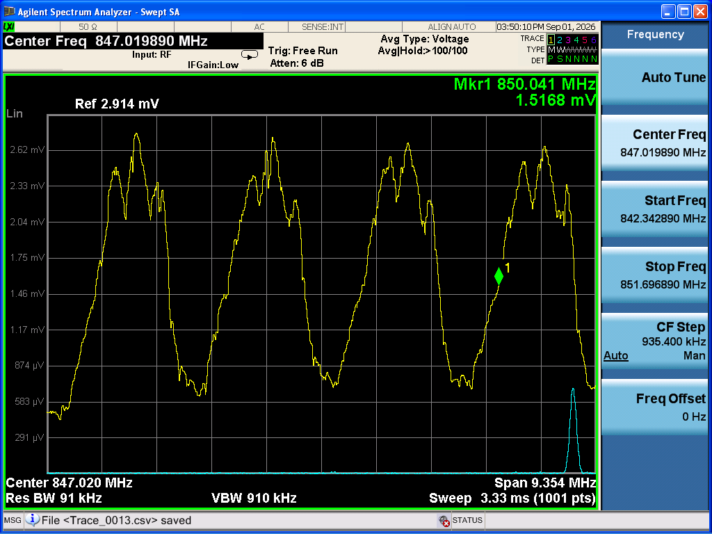
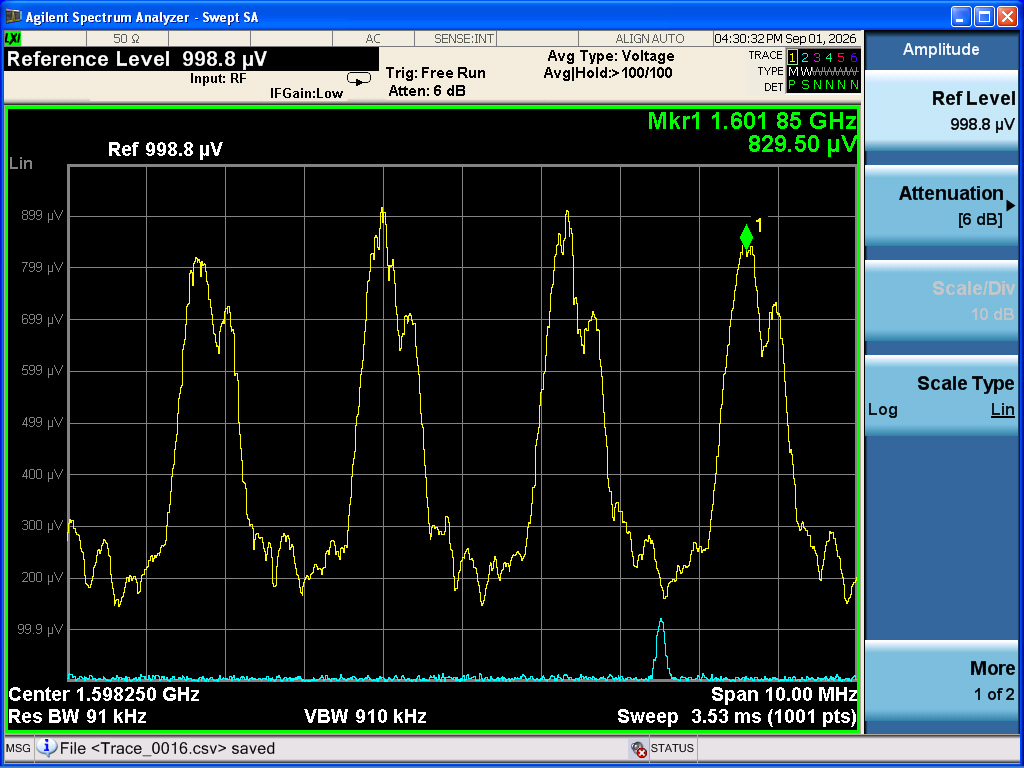
• When the measurement was first performed with S-polarization, the HWP setting was 82. By changing the HWP setting to 14 and the polarizer setting in front of the RFPD to 295, we were able to maximize the peak that was smaller in the initial S-polarization measurement. We then acquired data at beat frequencies of 1.6 GHz (Photo 3), 0.8 GHz (Photo 4), -0.8 GHz (Photo 5), and -1.6 GHz (Photo 6). Next, we set the HWP to 59 and the polarizer in front of the RFPD to 250, which allowed us to maximize the other peak. We then acquired data in the same way at beat frequencies of 1.6 GHz (Photo 7), 0.8 GHz (Photo 8), -0.8 GHz (Photo 9), and -1.6 GHz (Photo 10). The amplitudes of the beat signals when each peak was maximized were approximately 931 μV for the peak that was larger in the initial S-polarization measurement and approximately 1.46 mV for the peak that was smaller. Thus, the two peak amplitudes differed by a factor of approximately 1.57. In addition, when the HWP setting was 14, we checked the polarization of the sub-laser using a PBS. The measured powers were approximately 476 mW for P-polarization and 513 mW for S-polarization. Finally, we removed the HWP, but the beat signal was still split into two peaks, similar to the observation in Photo 2.

  The result of determining the SRY length from the data analysis will be posted later.

[Fujimoto, Ye, Saito]

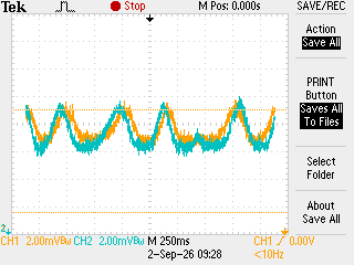
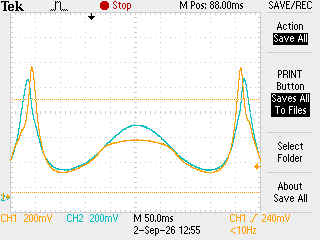
To investigate whether the splitting of the peak observed in the previous measurement (klog:37440) was caused by mode splitting due to birefringence of the ITM substrate, we used an HWP and a PBS to separate the light into S- and P-polarizations and installed PDs to monitor the two signals. When we performed cavity scans using only the main laser or only the sub-laser, we confirmed that the resonance positions of the cavity scans were different between S- and P-polarizations in both cases. Therefore, we consider that the splitting of the peak was caused by mode splitting due to birefringence of the ITM substrate.
 

• In the previous measurement (klog:37440), to investigate whether the splitting of the peak was caused by mode splitting due to birefringence of the ITM substrate, we placed an additional mirror after the mirror at the reflection port of OMMT2. We then placed an HWP and a PBS after this mirror and installed two PDs to monitor both the reflected and transmitted light from the PBS (Photo 1).
   
• Next, we rotated the HWP so that the transmitted and reflected powers from the PBS were approximately equal. The scale reading was 56, and both powers were approximately 0.7 mW. This scale reading was similar to the value obtained when the polarization was rotated by 45 degrees in the previous measurement (klog:37440).
   
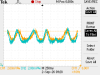
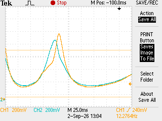
• We then turned off the main laser, removed the ND filter, and injected only the sub-laser in the S-polarization state. By sweeping the PZT with a triangular waveform, we confirmed that the resonance positions of the cavity scans were different between S- and P-polarizations (Photo 2). The orange line in Photo 2 shows the S-polarization signal, while the blue line shows the P-polarization signal. Since the relative shift reverses at the turning points of the triangular waveform, we consider that this is caused by mode splitting due to birefringence of the ITM substrate.
   
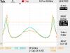
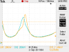
• Next, we turned off the sub-laser and used only the main laser. When we swept the SRM, we similarly observed a difference in the resonance positions between S- and P-polarizations (Photo 3). However, near each peak, the other polarization signal became smaller (Photo 4), suggesting that the S- and P-polarizations were not completely separated. We therefore rotated the HWP to see whether the two polarizations could be separated more completely, but there was no improvement. Therefore, the light appears to be elliptically polarized. The reason why this behavior was not observed when using the sub-laser is likely that the SNR was too low.

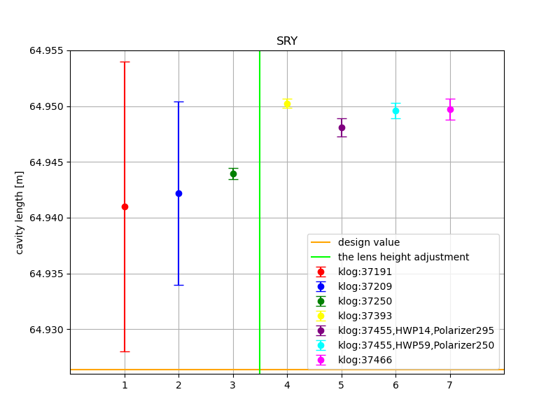
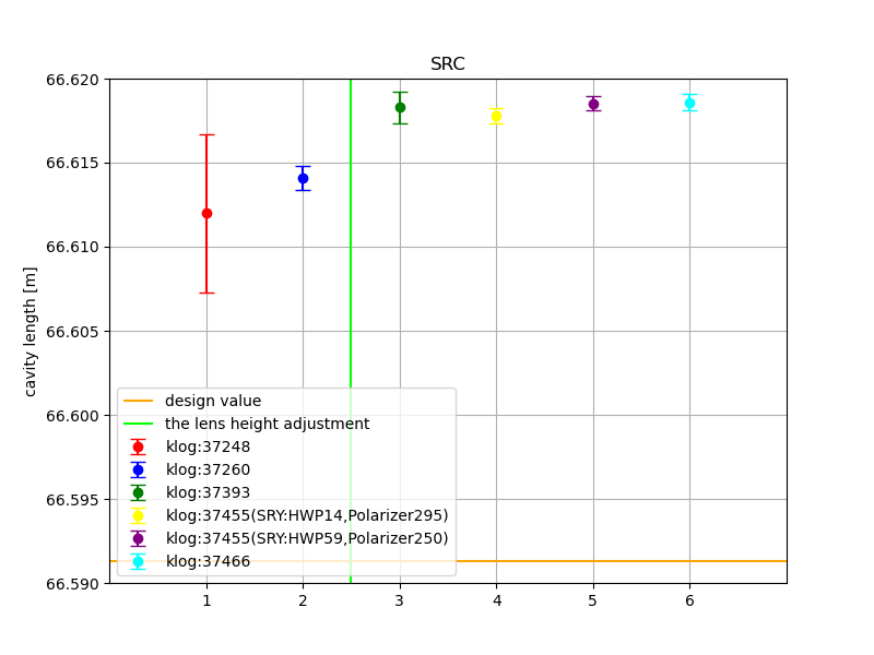
We analyzed the SRY data obtained in klog:37440. The deviation from the design value was 2.168(80) cm when the HWP scale was 14 and the polarizer scale was 295, and 2.319(71) cm when the HWP scale was 59 and the polarizer scale was 250. Compared with the previous measurement (klog:37393), which gave a deviation of 2.385(42) cm from the SRY design value, the result with the HWP scale at 59 is consistent, while the result with the HWP scale at 14 appears to be slightly different. Both results differ more significantly from the result before moving the lens to improve the mode-matching ratio (klog:37250), which gave a deviation of 1.757(50) cm from the design value.

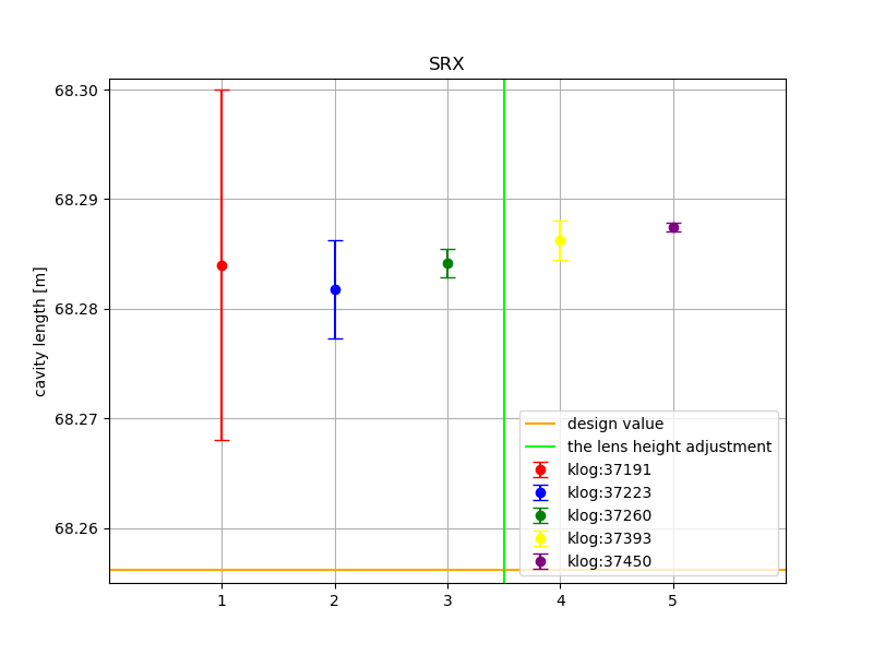
Using the SRX result from klog:37450, we also calculated the SRC length and the Schnupp asymmetry. The SRC lengths were 66.61778(45) m for the HWP scale of 14 and polarizer scale of 295, and 66.61853(41) m for the HWP scale of 59 and polarizer scale of 250. The Schnupp asymmetries calculated from the SRC lengths were 3.339390(904) m and 3.337880(825) m, respectively. Compared with the previous measurement (klog:37393), which gave an SRC length of 66.61828(92) m and a Schnupp asymmetry calculated from the SRC of 3.33605(185) m, both SRC lengths are consistent, while the Schnupp asymmetry with the HWP scale at 14 appears to be slightly different. Compared with the results before moving the lens to improve the mode-matching ratio (klog:37260), which gave an SRC length of 66.61409(70) m and a Schnupp asymmetry calculated from the SRC of 3.34023(139) m, both SRC lengths are slightly different, while the Schnupp asymmetry with the HWP scale at 59 appears to be slightly different.
 

• We fitted the SRY data obtained in klog:37440 with and without a linear background. I will post the fitting results for the individual peaks later. From the peak frequencies obtained from the fits and their uncertainties, we calculated the minimum and maximum values within the uncertainty ranges. We then took the overall minimum and maximum values from both fitting models, with and without a linear background, as the uncertainty range. The following data were therefore used to determine the SRY length.

  HWP scale: 14, Polarizer scale: 295
  Minimum (MHz)    Maximum (MHz)
  1611.7206    1611.8190
  810.9479    811.0371
  -846.1329    -845.9886
  -1656.2458    -1656.2199

  HWP scale: 59, Polarizer scale: 250
  Minimum (MHz)    Maximum (MHz)
  1599.4960    1599.5586
  789.4376    789.4956
  -814.5555    -814.4679
  -1583.0683    -1583.0217

  We set the FSR index of the data around -1.6 GHz to 0. For each pair of nearby peak frequencies, we calculated the frequency difference and divided it by the design value of the FSR. We then rounded the resulting value to the nearest integer to determine the FSR index. We fitted the measured peak frequencies as a function of the FSR index using the linear function AN+B, where A and B are fitting parameters and N is the FSR index.

  The fitting results were as follows.

  HWP scale: 14, Polarizer scale: 295 (Fig. 1)
  A: 2.307939(29) MHz
  B: -1656.230(13) MHz
  HWP scale: 59, Polarizer scale: 250 (Fig. 2)
  A: 2.307886(26) MHz
  B: -1583.043(22) MHz

  Since A corresponds to the FSR, we calculated the SRY length from the fitted value of A. The results were as follows.

  HWP scale: 14, Polarizer scale: 295
  Fitted length: 64.94808(80) m
  Design value: 64.9264 m
  Difference from the design value (fitted length − design value): 2.168(80) cm
  HWP scale: 59, Polarizer scale: 250
  Fitted length: 64.94959(71) m
  Design value: 64.9264 m
  Difference from the design value (fitted length − design value): 2.319(71) cm

  Compared with the previous measurement (klog:37393), which gave a deviation of 2.385(42) cm from the SRY design value, the result with the HWP scale at 59 is consistent, while the result with the HWP scale at 14 appears to be slightly different. Both results differ more significantly from the result before moving the lens to improve the mode-matching ratio (klog:37250), which gave a deviation of 1.757(50) cm from the design value.
   

• Using the SRX result from klog:37450, we calculated the SRC length and the Schnupp asymmetry as follows.

  HWP scale: 14, Polarizer scale: 295
  SRC
  Calculated value: 66.61778(45) m
  Design value: 66.5913 m
  Difference from the design value (calculated value − design value): 2.648(45) cm

  Schnupp asymmetry calculated from the SRC
  Calculated value: 3.339390(904) m
  Design value: 3.3298 m
  Difference from the design value (calculated value − design value): 0.9590(904) cm

  HWP scale: 59, Polarizer scale: 250
  SRC
  Calculated value: 66.61853(41) m
  Design value: 66.5913 m
  Difference from the design value (calculated value − design value): 2.723(41) cm

  Schnupp asymmetry calculated from the SRC
  Calculated value: 3.337880(825) m
  Design value: 3.3298 m
  Difference from the design value (calculated value − design value): 0.8080(825) cm

  Compared with the previous measurement (klog:37393), which gave an SRC length of 66.61828(92) m and a Schnupp asymmetry calculated from the SRC of 3.33605(185) m, both SRC lengths are consistent, while the Schnupp asymmetry with the HWP scale at 14 appears to be slightly different. Compared with the results before moving the lens to improve the mode-matching ratio (klog:37260), which gave an SRC length of 66.61409(70) m and a Schnupp asymmetry calculated from the SRC of 3.34023(139) m, both SRC lengths are slightly different, while the Schnupp asymmetry with the HWP scale at 59 appears to be slightly different.

The fitting results for the SRY measurements in klog:37455, with the HWP scale at 14 and the polarizer scale at 295, and with the HWP scale at 59 and the polarizer scale at 250, are shown below.

The measurement data are saved in the following Dropbox folders:

All files/Dropbox KAGRA/Measurements/IFO/SRCL/SRCL_OMMT2_REFL_beat_signal_PZT_sweep/2026_09_01_SRY_hwp14_pol295
All files/Dropbox KAGRA/Measurements/IFO/SRCL/SRCL_OMMT2_REFL_beat_signal_PZT_sweep/2026_09_01_SRY_hwp59_pol250
 

• HWP scale: 14, Polarizer scale: 295

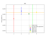
  Fig. 1: Around 1.6 GHz, without a linear background. Using the data from 1611.21 MHz to 1612.42 MHz, the fitted peak frequency was 1611.809(10) MHz.
  Fig. 2: Around 1.6 GHz, with a linear background. Using the data from 1611.21 MHz to 1612.42 MHz, the fitted peak frequency was 1611.766(45) MHz.

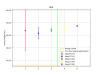
  Fig. 3: Around 800 MHz, without a linear background. Using the data from 810.37 MHz to 811.56 MHz, the fitted peak frequency was 810.962(11) MHz.
  Fig. 4: Around 800 MHz, with a linear background. Using the data from 810.37 MHz to 811.56 MHz, the fitted peak frequency was 810.993(45) MHz.

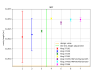
  Fig. 5: Around -800 MHz, without a linear background. Using the data from 845.47648 MHz to 846.683146 MHz, the fitted peak frequency was 846.1233(96) MHz.
  Fig. 6: Around -800 MHz, with a linear background. Using the data from 845.47648 MHz to 846.683146 MHz, the fitted peak frequency was 846.033(45) MHz.

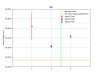
  Fig. 7: Around -1.6 GHz, without a linear background. Using the data from 1655.6 MHz to 1656.77 MHz, the fitted peak frequency was 1656.233(13) MHz.
  Fig. 8: Around -1.6 GHz, with a linear background. Using the data from 1656.6 MHz to 1656.77 MHz, the fitted peak frequency was 1656.2322(79) MHz.
   

• HWP scale: 59, Polarizer scale: 250

  Fig. 9: Around 1.6 GHz, without a linear background. Using the data from 1599.24 MHz to 1600.04 MHz, the fitted peak frequency was 1599.5509(77) MHz.
  Fig. 10: Around 1.6 GHz, with a linear background. Using the data from 1599.24 MHz to 1600.04 MHz, the fitted peak frequency was 1599.507(11) MHz.

  Fig. 11: Around 800 MHz, without a linear background. Using the data from 789.2 MHz to 789.96 MHz, the fitted peak frequency was 789.4894(61) MHz.
  Fig. 12: Around 800 MHz, with a linear background. Using the data from 789.2 MHz to 789.96 MHz, the fitted peak frequency was 789.449(11) MHz.

  Fig. 13: Around -800 MHz, without a linear background. Using the data from 814.0 MHz to 814.82 MHz, the fitted peak frequency was 814.4756(78) MHz.
  Fig. 14: Around -800 MHz, with a linear background. Using the data from 814.0 MHz to 814.82 MHz, the fitted peak frequency was 814.541(15) MHz.

  Fig. 15: Around -1.6 GHz, without a linear background. Using the data from 1582.56 MHz to 1583.35 MHz, the fitted peak frequency was 1583.0282(66) MHz.
  Fig. 16: Around -1.6 GHz, with a linear background. Using the data from 1582.56 MHz to 1583.35 MHz, the fitted peak frequency was 1583.0585(99) MHz.

[Fujimoto, Ye, Saito]

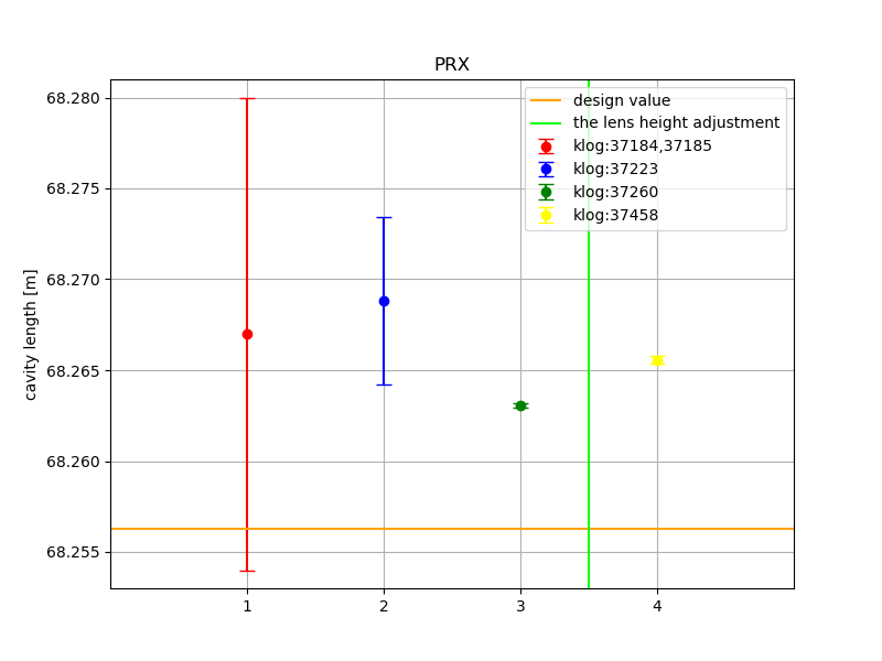
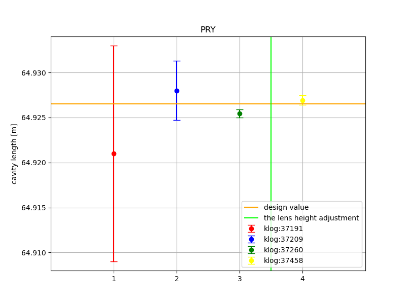
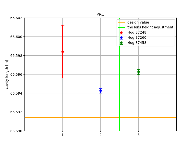
We adjusted the HWP and polarizer to obtain clean peaks and acquired beat signal data for PRX and PRY. After fitting the data, the deviations from the design values were 0.926(22) cm for PRX and 0.043(52) cm for PRY. Compared with the previous measurements before moving the lens to improve the mode-matching ratio (klog:37260), which gave deviations of 0.677(11) cm for PRX and -0.107(46) cm for PRY, both results are slightly different.

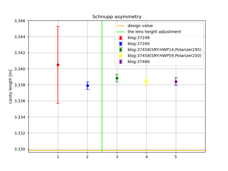
We also calculated the PRC length and the Schnupp asymmetry from the PRC. Using the Schnupp asymmetry calculated from the SRC in klog:37455, we then calculated the Schnupp asymmetry by taking a weighted average of the two values. The results were as follows:

PRC length: 66.59625(28) m
Schnupp asymmetry calculated from the PRC: 3.338630(565) m
Schnupp asymmetry from the weighted average:
3.33884(48) m when SRY was measured with the HWP scale at 14 and the polarizer scale at 295
3.33839(47) m when SRY was measured with the HWP scale at 59 and the polarizer scale at 250

Compared with the previous measurements before moving the lens to improve the mode-matching ratio (klog:37260), which gave a PRC length of 66.59425(24) m, a Schnupp asymmetry calculated from the PRC of 3.337640(473) m, and a Schnupp asymmetry from the weighted average of 3.33791(45) m, the PRC length is slightly different. However, there is no inconsistency between the Schnupp asymmetry calculated from the PRC and that calculated from the weighted average.
 

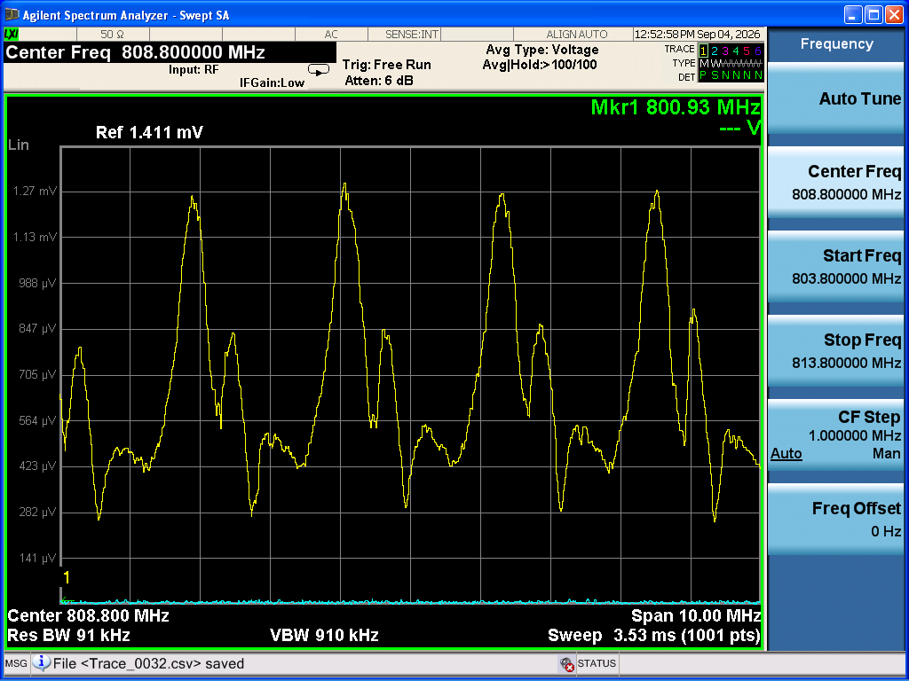
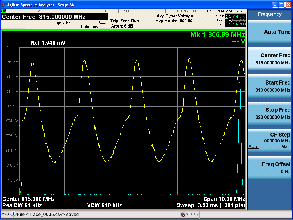
• To acquire the beat signal data for PRX, we first turned off the main laser and adjusted the alignment of the sub-laser. We then turned on the main laser and adjusted the alignment to the RFPD. When we checked the beat signal with the HWP scale at 82 and the polarizer scale at 50 using a spectrum analyzer, the peak was not clean (Photo 1). We therefore rotated the HWP and polarizer. The peak became clean when the HWP scale was set to 70 and the polarizer scale was set to 254. We then acquired data around 1.6 GHz (Photo 2), 0.8 GHz (Photo 3), -0.8 GHz (Photo 4), and -1.6 GHz (Photo 5).
   
• Similarly, for PRY, we first turned off the main laser and adjusted the alignment of the sub-laser. We then turned on the main laser and adjusted the alignment to the RFPD. We set the HWP scale to 16 and the polarizer scale to 117 to obtain clean peaks, and acquired data around 1.6 GHz (Photo 6), 0.8 GHz (Photo 7), -0.8 GHz (Photo 8), and -1.6 GHz (Photo 9).
   

• We then fitted the obtained PRX and PRY data with and without a linear background. I will post the fitting results for the individual peaks later. From the peak frequencies obtained from the fits and their uncertainties, we calculated the minimum and maximum values within the uncertainty ranges. We then took the overall minimum and maximum values from both fitting models, with and without a linear background, as the uncertainty range. The following data were therefore used to determine the PRX and PRY lengths.

  PRX
  Minimum (MHz)    Maximum (MHz)
  1591.7738    1591.8070
  807.8792    807.8958
  -821.3516    -821.3318
  -1563.5557    -1563.5479

  PRY
  Minimum (MHz)    Maximum (MHz)
  1600.1604    1600.1846
  810.5910    810.6133
  -817.0346    -816.9907
  -1597.4175    -1597.3530

  We set the FSR index of the data around -1.6 GHz to 0. For each pair of nearby peak frequencies, we calculated the frequency difference and divided it by the design value of the FSR. We then rounded the resulting value to the nearest integer to determine the FSR index. We fitted the measured peak frequencies as a function of the FSR index using the linear function AN+B, where A and B are fitting parameters and N is the FSR index.

  The fitting results were as follows.

  PRX (Fig. 1)
  A: 2.1957810(72) MHz
  B: -1563.5483(38) MHz

  PRY (Fig. 2)
  A: 2.308691(19) MHz
  B: -1597.363(21) MHz

  Since A corresponds to the FSR, we calculated the PRX and PRY lengths from the fitted values of A. The results were as follows.

  PRX
  Fitted length: 68.26556(22) m
  Design value: 68.2563 m
  Difference from the design value (fitted length − design value): 0.926(22) cm

  PRY
  Fitted length: 64.92693(52) m
  Design value: 64.9265 m
  Difference from the design value (fitted length − design value): 0.043(52) cm

  Compared with the previous measurements before moving the lens to improve the mode-matching ratio (klog:37260), which gave deviations of 0.677(11) cm for PRX and -0.107(46) cm for PRY, both results are slightly different.
   

• We also calculated the PRC length and the Schnupp asymmetry from the PRC. Using the Schnupp asymmetry calculated from the SRC in klog:37455, we calculated the Schnupp asymmetry from the weighted average as follows.

  PRC
  Calculated value: 66.59625(28) m
  Design value: 66.5914 m
  Difference from the design value (calculated value − design value): 0.485(28) cm

  Schnupp asymmetry calculated from the PRC
  Calculated value: 3.338630(565) m
  Design value: 3.3298 m
  Difference from the design value (calculated value − design value): 0.8830(565) cm

  Schnupp asymmetry
  When SRY was measured with the HWP scale at 14 and the polarizer scale at 295:
  Weighted average: 3.33884(48) m
  Design value: 3.3298 m
  Difference from the design value (weighted average − design value): 0.904(48) cm

  When SRY was measured with the HWP scale at 59 and the polarizer scale at 250:
  Weighted average: 3.33839(47) m
  Design value: 3.3298 m
  Difference from the design value (weighted average − design value): 0.859(47) cm

  Compared with the previous measurements before moving the lens to improve the mode-matching ratio (klog:37260), which gave a PRC length of 66.59425(24) m, a Schnupp asymmetry calculated from the PRC of 3.337640(473) m, and a Schnupp asymmetry from the weighted average of 3.33791(45) m, the PRC length is slightly different. However, there is no inconsistency between the Schnupp asymmetry calculated from the PRC and that calculated from the weighted average.

The fitting results for PRX and PRY in klog:37458 are shown below.
The measurement data are saved in the following Dropbox folders:

All files/Dropbox KAGRA/Measurements/IFO/PRCL/PRCL_OMMT2_REFL_beat_signal_PZT_sweep/2026_09_04_PRX
All files/Dropbox KAGRA/Measurements/IFO/PRCL/PRCL_OMMT2_REFL_beat_signal_PZT_sweep/2026_09_04_PRY
 

• PRX
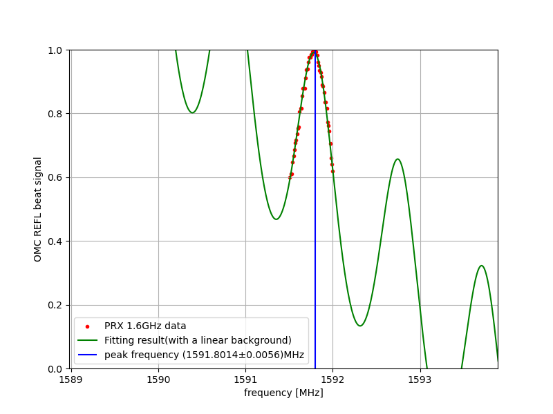
  Fig. 1: Around 1.6 GHz, without a linear background. Using the data from 1591.51 MHz to 1592.0 MHz, the fitted peak frequency was 1591.7750(12) MHz.
  Fig. 2: Around 1.6 GHz, with a linear background. Using the data from 1591.51 MHz to 1592.0 MHz, the fitted peak frequency was 1591.8014(56) MHz.

  Fig. 3: Around 800 MHz, without a linear background. Using the data from 807.62 MHz to 808.15 MHz, the fitted peak frequency was 807.8942(17) MHz.
  Fig. 4: Around 800 MHz, with a linear background. Using the data from 807.62 MHz to 808.15 MHz, the fitted peak frequency was 807.8842(49) MHz.

  Fig. 5: Around -800 MHz, without a linear background. Using the data from 821.12 MHz to 821.59 MHz, the fitted peak frequency was 821.3504(11) MHz.
  Fig. 6: Around -800 MHz, with a linear background. Using the data from 821.12 MHz to 821.59 MHz, the fitted peak frequency was 821.3352(35) MHz.

  Fig. 7: Around -1.6 GHz, without a linear background. Using the data from 1563.29 MHz to 1563.82 MHz, the fitted peak frequency was 1563.5494(14) MHz.
  Fig. 8: Around -1.6 GHz, with a linear background. Using the data from 1563.29 MHz to 1563.82 MHz, the fitted peak frequency was 1563.5525(32) MHz.
   

• PRY
  Fig. 9: Around 1.6 GHz, without a linear background. Using the data from 1599.85 MHz to 1600.57 MHz, the fitted peak frequency was 1600.1828(18) MHz.
  Fig. 10: Around 1.6 GHz, with a linear background. Using the data from 1599.85 MHz to 1600.57 MHz, the fitted peak frequency was 1600.1637(33) MHz.

  Fig. 11: Around 800 MHz, without a linear background. Using the data from 810.32 MHz to 810.95 MHz, the fitted peak frequency was 810.6120(14) MHz.
  Fig. 12: Around 800 MHz, with a linear background. Using the data from 810.32 MHz to 810.95 MHz, the fitted peak frequency was 810.5939(29) MHz.

  Fig. 13: Around -800 MHz, without a linear background. Using the data from 816.67 MHz to 817.23 MHz, the fitted peak frequency was 816.9934(28) MHz.
  Fig. 14: Around -800 MHz, with a linear background. Using the data from 816.67 MHz to 817.23 MHz, the fitted peak frequency was 817.0274(72) MHz.

  Fig. 15: Around -1.6 GHz, without a linear background. Using the data from 1596.96 MHz to 1597.66 MHz, the fitted peak frequency was 1597.3557(27) MHz.
  Fig. 16: Around -1.6 GHz, with a linear background. Using the data from 1596.96 MHz to 1597.66 MHz, the fitted peak frequency was 1597.4093(82) MHz.

[Fujimoto, Saito]

We adjusted the HWP and polarizer for SRY to obtain a clean peak and acquired the beat signal data. After fitting the data, the deviation of the SRY length from the design value was found to be 2.332(93) cm. This result is consistent with the previous measurements reported in klog:37455: the deviations from the design value were 2.168(80) cm with the HWP scale at 14 and the polarizer scale at 295, and 2.319(71) cm with the HWP scale at 59 and the polarizer scale at 250. However, it is slightly different from the result obtained before moving the lens to improve the mode-matching ratio (klog:37250), where the deviation of the SRY length from the design value was 1.757(50) cm.

Using the SRX result from klog:37450 and the results from klog:37458, I calculated the SRC length and Schnupp asymmetry as follows:

SRC length: 66.61860(51) m
Schnupp asymmetry calculated from the SRC: 3.33775(102) m
Schnupp asymmetry from the weighted average: 3.33842(49) m

These results are consistent with the previous measurements reported in klog:37455 and klog:37458. With the HWP scale at 14 and the polarizer scale at 295, the SRC length was 66.61778(45) m, the Schnupp asymmetry calculated from the SRC was 3.339390(904) m, and the Schnupp asymmetry from the weighted average was 3.33884(48) m. With the HWP scale at 59 and the polarizer scale at 250, the corresponding values were 66.61853(41) m, 3.337880(825) m, and 3.33839(47) m, respectively. Comparing these results with the measurements before moving the lens to improve the mode-matching ratio (klog:37260), where the SRC length was 66.61409(70) m, the Schnupp asymmetry calculated from the SRC was 3.34023(139) m, and the Schnupp asymmetry from the weighted average was 3.33791(45) m, the SRC length and the Schnupp asymmetry calculated from the SRC are somewhat different. However, the Schnupp asymmetry obtained from the weighted average is consistent with the previous result.
 

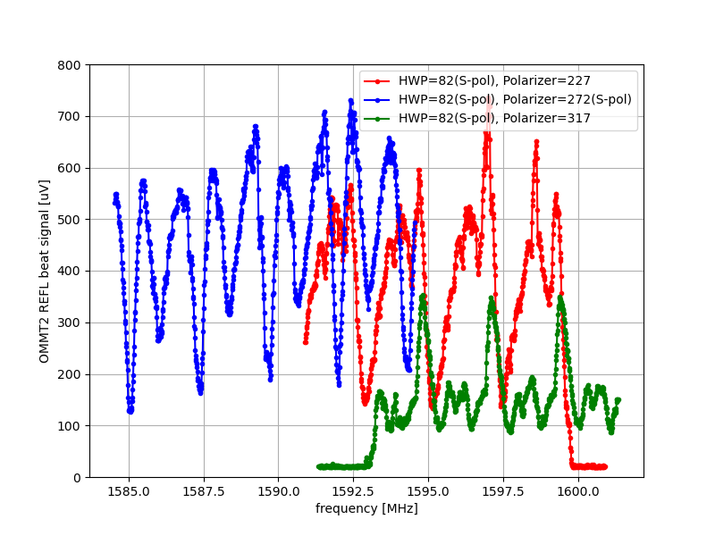
• First, we set the HWP scale at the sub-laser to 82 (S polarization) and set the polarizer in front of the RFPD to S polarization. With the main laser turned off, we adjusted the alignment of the sub-laser to SRY. Next, we locked the main laser to SRY, adjusted the alignment to the RFPD, and checked the beat signal. However, as in the previous measurement (klog:37440), the peak was split. Therefore, we adjusted the alignment of the sub-laser to maximize the beat signal, and rotated the HWP and polarizer to maximize the beat signal as well. The HWP scale was then 124 (P polarization), and the polarizer scale was 2 (P polarization). However, the peak was split into three peaks.

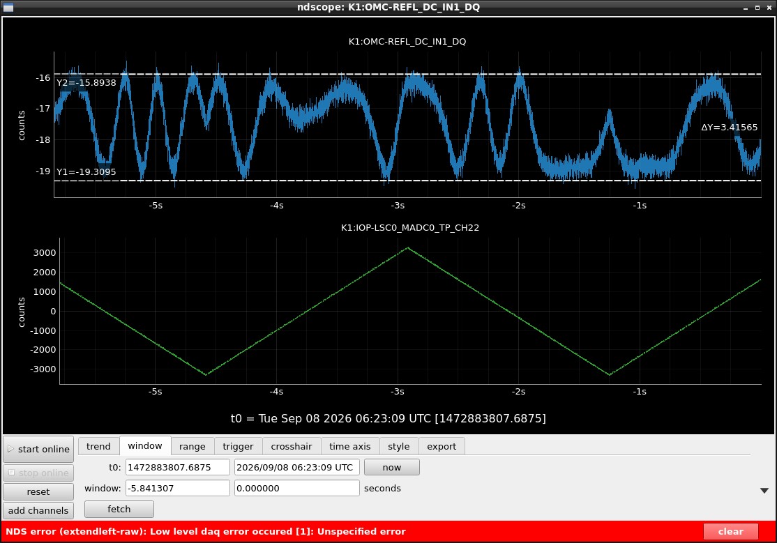
  Next, we turned off the main laser and adjusted the alignment again using the sub-laser. When the polarizer in front of the RFPD was removed, the maximum signal was -16 counts for S-polarized injection and -52 counts for P-polarized injection, giving a difference of about a factor of three. The peak also appeared cleaner as a single peak for S polarization, whereas it was split into about three peaks for P polarization.

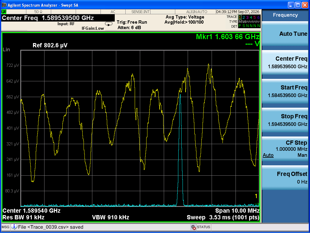
  Next, with the HWP scale at 82 (S polarization), we set the polarizer scale to 272 (S polarization). Peaks separated by approximately 1 MHz were observed (Photo 1). we then set the polarizer scale to 317, and one of the two peaks became larger (Photo 2). When I set the polarizer scale to 227, the other peak appeared to become larger (Photo 3). The three cases are plotted together in Fig. 1.
   

• Next, we acquired beat signal data around 1.6 GHz (Photo 4), 0.8 GHz (Photo 5), -0.8 GHz (Photo 6), and -1.6 GHz (Photo 7) with the HWP scale at 82 and the polarizer scale at 317, where the peak appeared the cleanest. I fitted the obtained SRY data both with and without a linear background. I will post the fitting results for the individual peaks later. From the peak frequencies obtained from the fits and their uncertainties, I calculated the minimum and maximum values within the uncertainty ranges. I then took the overall minimum and maximum values from the two fitting models, with and without a linear background, as the uncertainty range.
  Therefore, I used the following data to determine the SRY length:

  Minimum (MHz)    Maximum (MHz)
  1610.8271    1610.9060
  803.0776    803.1743
  -800.9112    -800.8258
  -1592.4969    -1592.4366

  I set the FSR index of the data around -1.6 GHz to 0. For each pair of nearby peak frequencies, I calculated the frequency difference and divided it by the design value of the FSR. I then rounded the resulting value to the nearest integer to determine the FSR index. I fitted the measured peak frequencies as a function of the FSR index using the linear function AN+B, where A and B are fitting parameters and N is the FSR index.
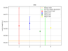
  The fitting results are shown below (Fig. 2):

  A: 2.307881(33) MHz
  B: -1592.467(27) MHz

  Since A corresponds to the FSR, I calculated the SRY length from the fitted value of A, obtaining:

  Fitted value: 64.94972(93) m
  Design value: 64.9264 m
  Difference from the design value (fitted value − design value): 2.332(93) cm

  This result is consistent with the previous measurements reported in klog:37455: the deviations from the design value were 2.168(80) cm with the HWP scale at 14 and the polarizer scale at 295, and 2.319(71) cm with the HWP scale at 59 and the polarizer scale at 250. However, it is slightly different from the result obtained before moving the lens to improve the mode-matching ratio (klog:37250), where the deviation of the SRY length from the design value was 1.757(50) cm.
   

• Using the SRX result from klog:37450 and the results from klog:37458, I calculated the SRC length and Schnupp asymmetry as follows:

  SRC
  Calculated value: 66.61860(51) m
  Design value: 66.5913 m
  Difference from the design value (calculated value − design value): 2.730(51) cm

  Schnupp asymmetry calculated from the SRC
  Calculated value: 3.33775(102) m
  Design value: 3.3298 m
  Difference from the design value (calculated value − design value): 0.795(102) cm

  Schnupp asymmetry
  Weighted average: 3.33842(49) m
  Design value: 3.3298 m
  Difference from the design value (weighted average − design value): 0.862(49) cm

  These results are consistent with the previous measurements reported in klog:37455 and klog:37458. With the HWP scale at 14 and the polarizer scale at 295, the SRC length was 66.61778(45) m, the Schnupp asymmetry calculated from the SRC was 3.339390(904) m, and the Schnupp asymmetry from the weighted average was 3.33884(48) m. With the HWP scale at 59 and the polarizer scale at 250, the corresponding values were 66.61853(41) m, 3.337880(825) m, and 3.33839(47) m, respectively. Compared with the measurements before moving the lens to improve the mode-matching ratio (klog:37260), where the SRC length was 66.61409(70) m, the Schnupp asymmetry calculated from the SRC was 3.34023(139) m, and the Schnupp asymmetry from the weighted average was 3.33791(45) m, the SRC length and the Schnupp asymmetry calculated from the SRC are somewhat different. However, the Schnupp asymmetry obtained from the weighted average is consistent with the previous result.

The fitting results for SRY in klog:37466 are shown below.

The measurement data are saved in the following Dropbox folder:

All files/Dropbox KAGRA/Measurements/IFO/SRCL/SRCL_OMMT2_REFL_beat_signal_PZT_sweep/2026_09_07_SRY
 

• Fig. 1: Around 1.6 GHz, without a linear background. Using data from 1610.59 MHz to 1611.02 MHz, the fitted peak frequency was 1610.8297(27) MHz.
  Fig. 2: Around 1.6 GHz, with a linear background. Using data from 1610.59 MHz to 1611.02 MHz, the fitted peak frequency was 1610.893(13) MHz.

  Fig. 3: Around 800 MHz, without a linear background. Using data from 802.82 MHz to 803.27 MHz, the fitted peak frequency was 803.0799(23) MHz.
  Fig. 4: Around 800 MHz, with a linear background. Using data from 802.82 MHz to 803.27 MHz, the fitted peak frequency was 803.147(27) MHz.

  Fig. 5: Around -800 MHz, without a linear background. Using data from 800.72 MHz to 801.16 MHz, the fitted peak frequency was 800.9089(24) MHz.
  Fig. 6: Around -800 MHz, with a linear background. Using data from 800.72 MHz to 801.16 MHz, the fitted peak frequency was 800.839(13) MHz.

  Fig. 7: Around -1.6 GHz, without a linear background. Using data from 1592.3195 MHz to 1592.7295 MHz, the fitted peak frequency was 1592.4944(25) MHz.
  Fig. 8: Around -1.6 GHz, with a linear background. Using data from 1592.3195 MHz to 1592.7295 MHz, the fitted peak frequency was 1592.4459(93) MHz.