Yesterday  I performed the calibration of the accelerometers on the ITMX IP, and after that I measured   and implemented the related sensing matrix. We remind that also the accelerometers are arranged in a plane geometry, on the vertices of an equilateral triangle (120 degrees between each to other and far from the center of IP r=0.5592 m).
 Here some details of this work are reported.

=Accelerometers calibration=

One way to do this calibration is to move the IP along the Yaw degree of freedom by  injecting white noise  and measure the transfer function: TF_yaw_acc_i= (Yaw_lvdt*r)./(acc_i)/(2*pi*f)^2 ) (where i=1,2,3);

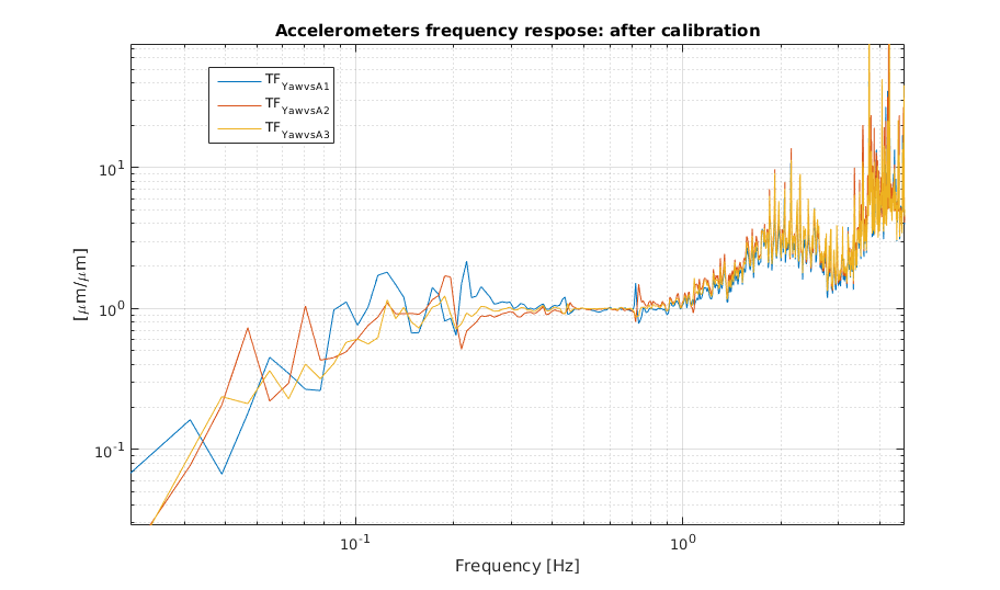
Since the Yaw is an isotropic motion I expect that the accelerometers read the same signal, that is: the functions TF_yaw_acc_i  must  be  equals. If this happens the sensors are calibrated, otherwise  we have to calibrate them.
For the ITMX I did this operation:
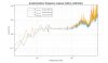
- In Fig1 is shown the  TF_yaw_acc_i before the calibration: we see that these responses are different each others.

At   0.5  these transfer functions assume the values reported below:

These values represent the calibration factors that we have to use to equalize the response between the accelerometers and LVDTs.
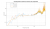
I uploted these new calibration factors in the MEDM screen and  measured agin the TF_yaw_acc_i:
- In Fig2 is shown the TF_yaw_acc_i  after the calibration: we see that these responses are equal.
 

=Accelerometers sensing matrix=

To built the diagonalized virtual accelerometers I  chosen to measure the sensing matrix referring at the readout of the diagonalized virtual sensors (L,T,Yaw). This measurement is done by injecting a line at with frequency f0 from each Virtual diagonalized actuator [CoilL, CoilT, CoilY] and by measuring module and phase of the transfer function between the j-th inertial sensor (in this case accelerometer) and the diagonalized LVDTs i=[L ,T ,Yaw]: TFji=(Acc_j/L_i)/(2*pi*f0)^2
 In this way it is possible to measure the amplitude of the response (module) and the sign(TF phase) that each  real inertial sensor has when we  move only along the selected degree of freedom . These numbers are stored for column in a matrix S whose the  inverse is the sensing matrix. A crucial point for the measurement of these matrices is the choice of the frequency f0. We reminde that we have to monitor very small displacements in  low frequency region (below 3 Hz), where the inertial sensor must have a good response. Looking at the frequency response (see Fig2) we see that the accelerometer response in the range [0.1 ,2.5] Hz is more or less linear, (this means that the their output is proportional to the acceleration of the IP), then it is appropriate to choose f0 in this range and far from the mechanical resonances of the system.  Since the last resonance of the chain is  at about 1 Hz, I choose to inject the line at  f0=2Hz.
Below is reported the accelerometers sensing matrix:

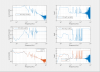
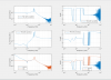
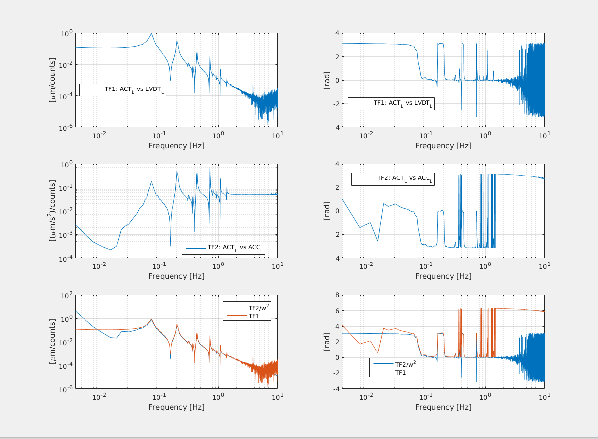
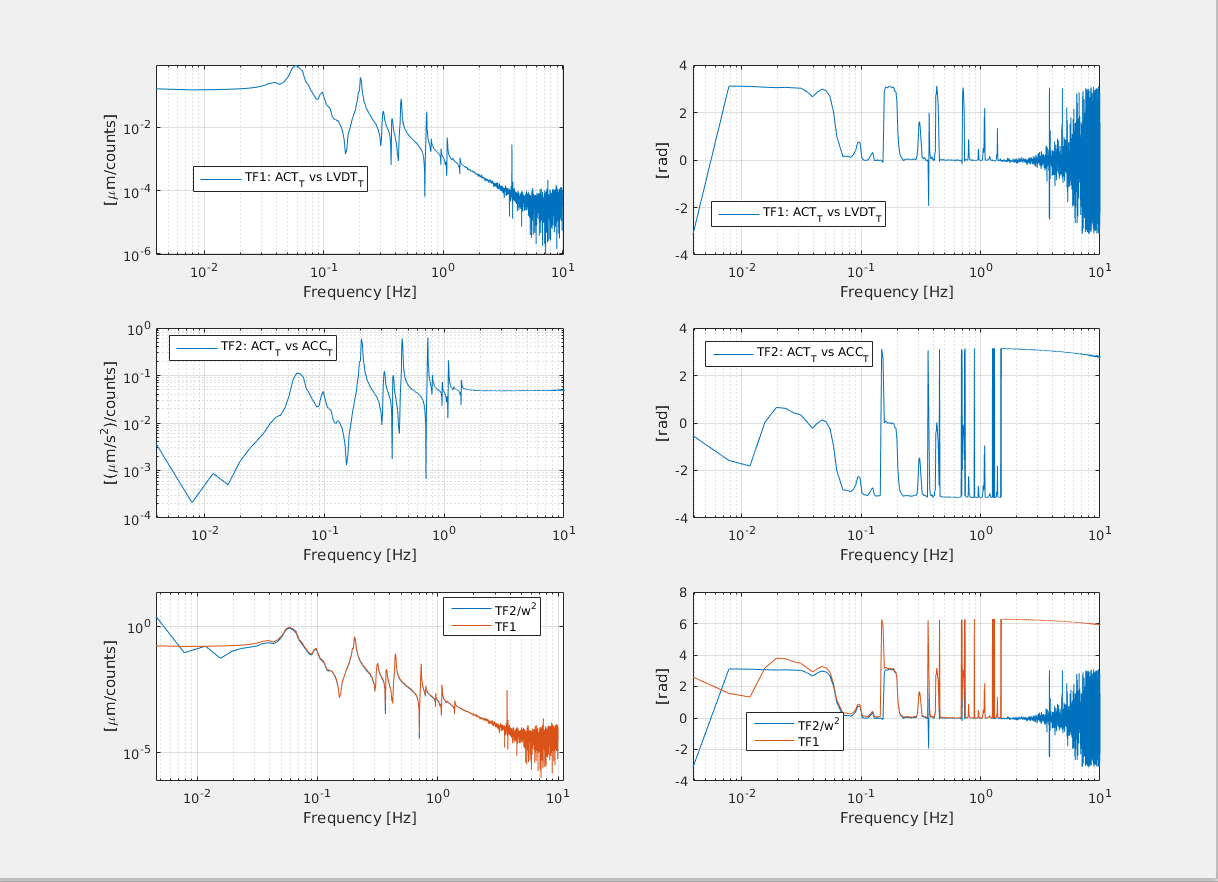
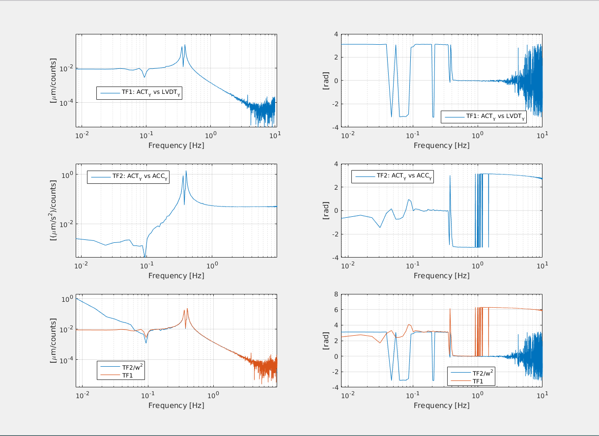
To check the goodness of  the calibration procedure and of this matrix   I measured the transfer functions by injecting white noise from diagonalized virtual actuators and looking at diagonalized virtual LVDTs  and Accelerometers: If the calibration factor and  matrix are correct I expect that the TF_lvdt=TF_acc/(w^2)
In the plot [Fig3,Fig4,Fig5] are shown these measurement and we can see that for all d.o.f is verified the assumption:F_lvdt=TF_acc/(w^2).