[Shih-Hong Hsu, Chia-Jui Chou, Hirotaka Yuzurihara, Yi Yang]

    This is an analysis report of the relation between seismic motion near BS (K1:PEM-SEIS_BS_GND_{X, Y, Z}_OUT_DQ) and the occurrence of scattered light noise in PRCL (JGW-G2416289). The data contains dates with lock segments longer than 1200 s in late February. The dates are 02/11, 18, 19-22. Note that from 02/19, the interferometer changed to a 10 W operation. (k-log 32748, 32756)

    The result shows a positive relation between the number of occurrences of scattered light noise in PRCL and seismic motion near BS (or PRCL). And before the 10 W operation, scattered light noise is more sensitive to seismic motion.
 

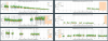
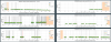
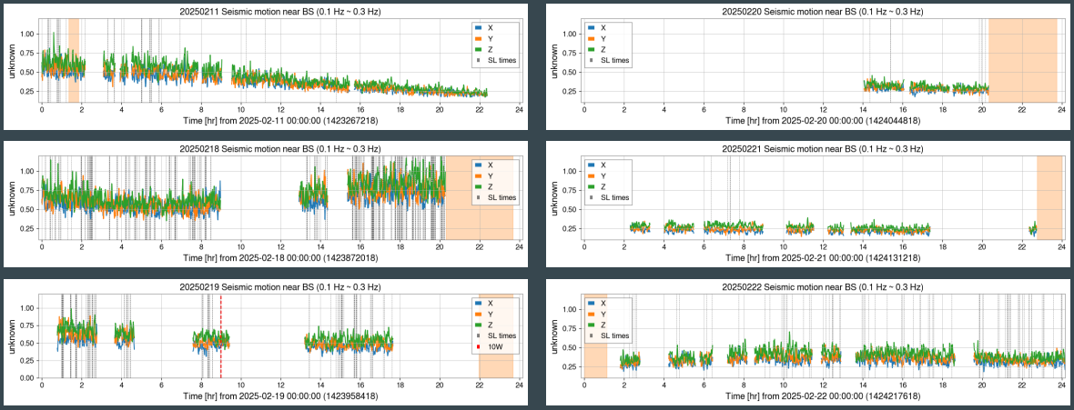
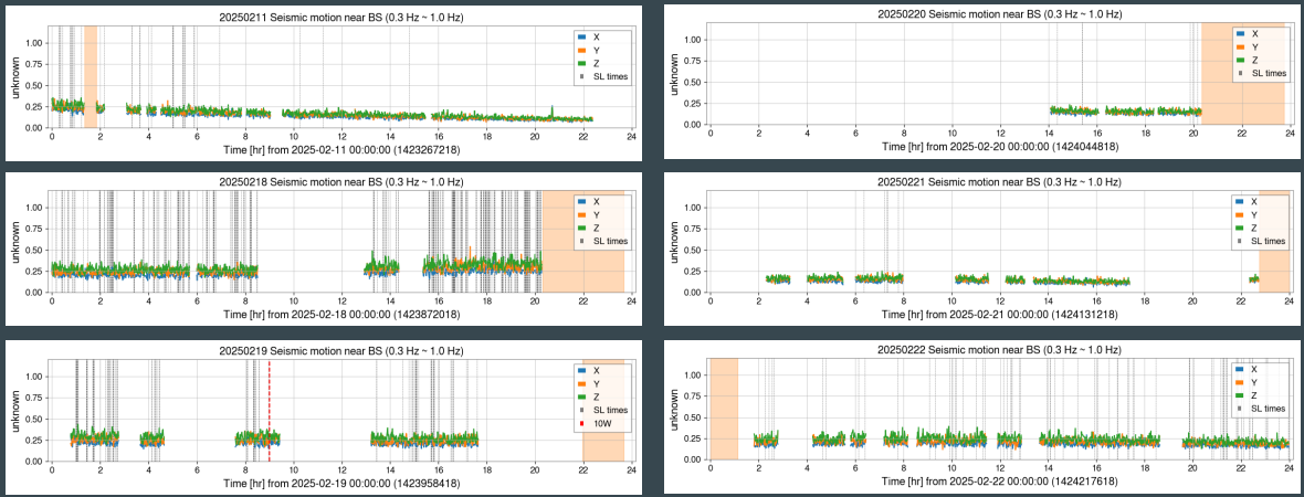
    First, I prepared the band-passed time series of the seismic motion near BS for 02/11, 02/18, 02/19, 02/20, 02/21, 02/22. The preparation contains 

• Check for any ongoing injection test in the interferometer by the k-log reports. If there is an injection test, I do not use the data. -> orange spans

• Label when the scattered light noise happened in PRCL (K1:LSC-PRCL_OUT_DQ). -> vertical black dotted lines (How I get the labels: JGW-G2416344)

• Check the 10 W operation start time, which is about at 02/19 09:00 UTC. -> vertical red dashed line.

I use the bands of 0.1 ~ 0.3 Hz and 0.3 ~ 1.0 Hz. The channel names are

• 0.1 ~ 0.3 Hz: K1:PEM-SEIS_BS_GND_{X, Y, Z}_BLRMS_100MHZ300.rms (Fig. 1)

• 0.3 ~ 1.0 Hz: K1:PEM-SEIS_BS_GND_{X, Y, Z}_BLRMS_300MHZ1000.rms (Fig. 2)

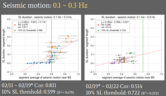
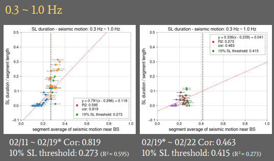
    Second, I divide the lock segments (K1:GRD-LSC_LOCK_STATE_N ≥ 9990) into subsegments with a length of 3600 s and count the number of the scattered light labels. Each label, t_i, represents the time between t_i and t_i + 30 s; one can see the scattered light (SL) noise in PRCL and |t_i - t_j| > 30 s for i ≠ j. Therefore, let N be the number of SLs; I use the ratio “ r = (N * 30) / 3600 ⇒ 0 ≤ r ≤ 1 “ to represent the amount of the occurrence of the SL in each hour subsegment.

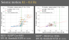
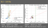
    Finally, I made the scatter plots for the SL occurrence w.r.t. average seismic motion of each point standing for a subsegment. I separated the scatter plots into groups of 0.1~0.3 Hz motion (Fig. 3) and 0.3~1 Hz (Fig. 4) and compared them before (left) and after (right) 10 W operation.

    As a result, the distribution of the scatter plots suggests a positive correlation between the SL occurrence and seismic motion strength. Thus, I used the least square method to linearly fit the data to give a naive threshold of seismic motion that SL occurrence r = 10%. From the magnitude of the slope, the SL occurrence is more sensitive to seismic motion.