[Akutsu, Ushiba, Michimura]

We have done oplev diagonalization for SRM. We basically reproduced the previous diagonalization matrix, and updated the matrix. The update matrix now ignores LEN_YAW signal.
It seems that it is important to use IP to excite longitudinal motion off the resonance, and avoid using pendulum mode frequency for the diagonalization.


What we did:
 0. Holded Oplev DC control outputs and turned off oplev loops by going to TWR_DAMPED state.

 1. Kicked SRM TM in L by adding 6000cnts to K1:VIS-SRM_TM_TEST_L_OFFSET.

 2. Measured the spectrum of K1:VIS-SRM_TM_OPLEV_LEN_PIT_OUT, K1:VIS-SRM_TM_OPLEV_TILT_PIT_OUT, K1:VIS-SRM_TM_OPLEV_TILT_YAW_OUT.

 3. Made the matrix:

SensMat = [[1, SL(fP)/SP(fP),SL(fY)/SY(fY)],[SP(fL)/SL(fL),1,SP(fY)/SY(fY)],[SY(fL)/SL(fL),SY(fP)/SP(fP),1]]

where SL, SP, SY are the spectrum of LEN, PIT, YAW, respectively, and fL, fP, fY are the natural resonant frequencies. Signs are

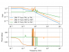
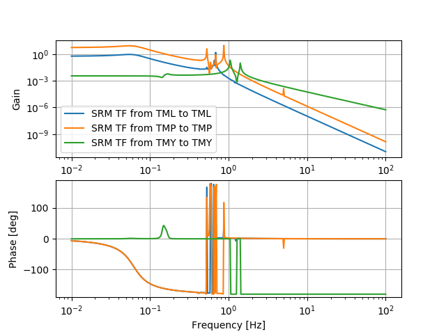
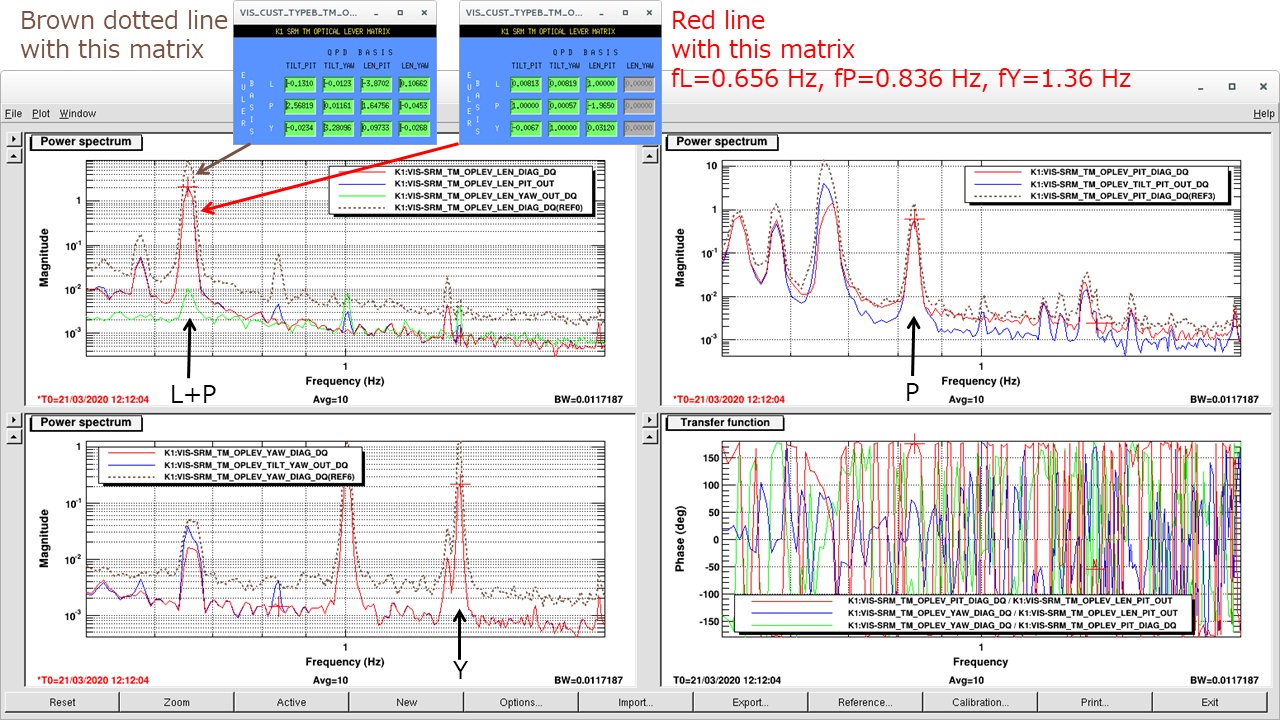
As for fL, fP, fY for SRM, we used 0.656 Hz, 0.836 Hz, 1.36 Hz (Thank you Terrence for the comments! See, also Fig. 1 from VIS Plotter).

 4. Inverted the matrix and normalized so that diagonal components will be 1.

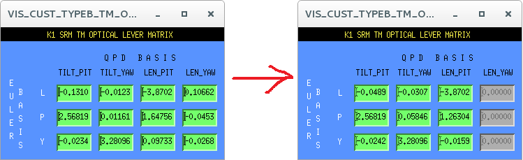
 5. Put them in the K1:VIS-SRM_TM_OPLEV_OL2EUL matrix.

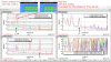
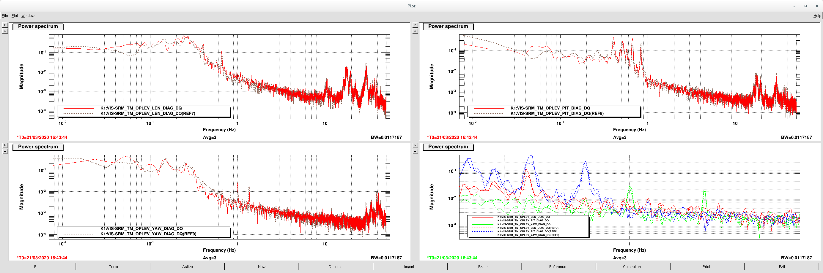
 6. Measured the oplev signal before OL2EUL matrix and after OL2EUL matrix. See Fig. 2. After OL2EUL matrix (red curves) have less contamination of other modes than before the matrix (blue curves). Dotted brown curves are signals after OL2EUL matrix, before our work. You can see some residual mixing of LEN motion to PIT and YAW, but seems to be better than the previous OL2EUL matrix.

 7. Re-normalized the OL2EUL matrix so that diagonal components will be the same as previous one. We decided not to make diagonal components 1 since we didn't want to change the calibration, and oplev damping filter gains.

 8. Turned back the oplev loops again and found that the loops will go crazy.

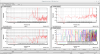
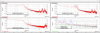
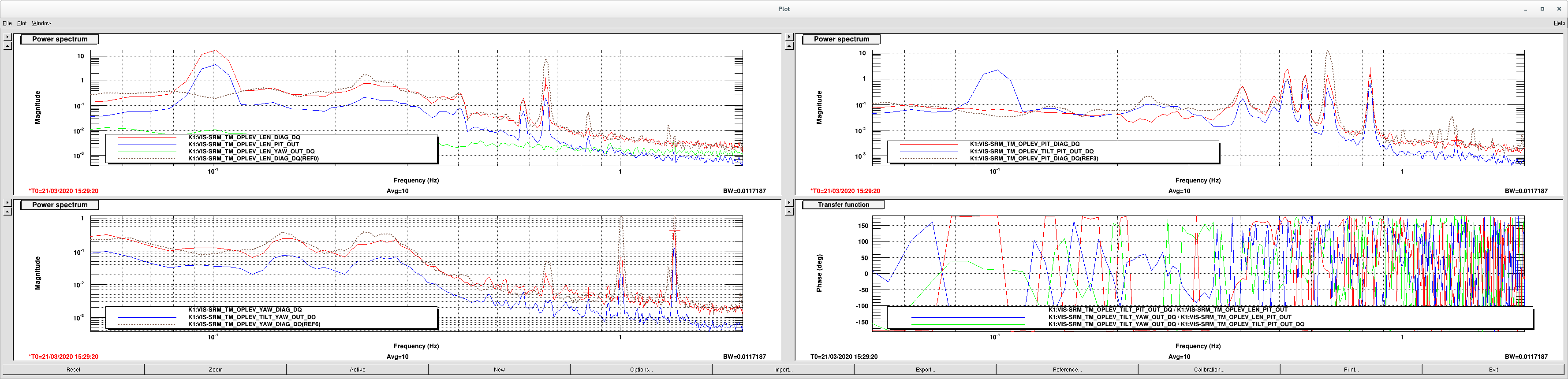
 9. So, I re-done the process by applying 0.1 Hz excitation with the amplitude of 10cnts to IP L from K1:VIS-SRM_IP_TEST_L_EXCMON, and calculate SensMat using fL=0.1 Hz. See Fig. 3 showing the ratio of LEN, PIT and YAW spectra and Fig. 4 before and after the diagonaization. Looks good.

 10. Turned back the oplev loops again and found that the loops are fine.

 11. Fig. 5 shows the oplev signals after diagonalization using previous OL2EUL matrix (in REFs) and new one, when oplev loops are turned off. The change is not so significant, but I will keep the updated matrix since we are more confortable not using LEN_YAW.

 12. Fig. 6 shows the comparison of previous and new OL2EUL matrix.

Discussion
 - We assumed QPD quadrant gains are well balanced.
 - In the method above, we assumed that LEN_YAW signal do not contain any signal. This can be justified by the fact that LEN_PIT has more length signal than LEN_YAW by more than two orders of magnitude (see green curve on top left plot).
 - You can see 1.1 Hz peak especcially in YAW. I think this is also from yaw motion (see attached TFs from VIS Plotter).
 - We discovered that there was a nice document by Terrence on oplev diagonalization of BS and SRs at JGW-T1910189.
 - We are aware that Oplev QPDs are not centered and out of range (+/- 50 according to Terrence), but we will use the updated matrix for now because we don't want to center it right now. Oplev diagonalization should be done again later after the centering.

Next:
 - Check oplev diagonalization of SR2 and SR3
 - Coil balancing of SRM, SR2 and SR3