Work of last week and this week:
Geophone Calibration
A long while ago, Lucia and I install the calibration filter of the SRM geophone.
I put an integrator and a DC cutoff (4th order high pass at 0.003 Hz) so the output of the geophone input filters gives unit in displacement.
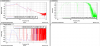
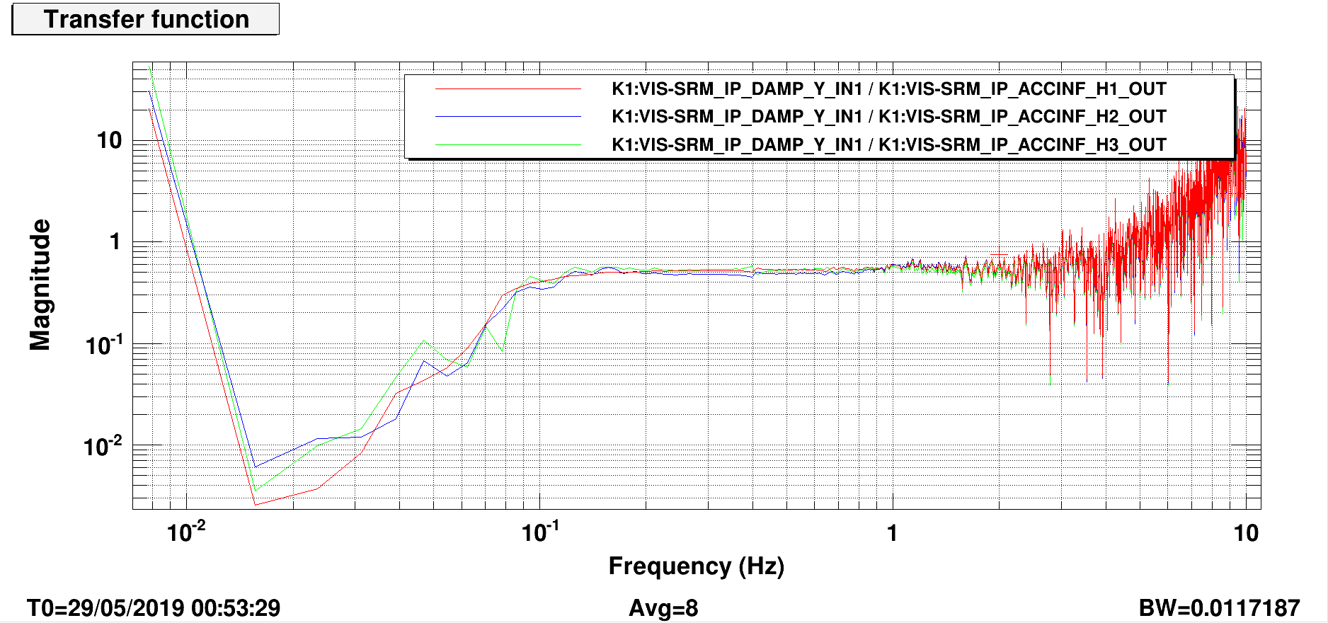
To filter calibrate the geophones, I put on yaw excitation and measured TFs (IP Yaw)/(Gi), where Gi is the i th geophone output. See figure 1. From the yaw readout and the distance from the center to the geophones, we can calculate the tangential displacement. Conventionally, Lucia chooses 0.5 Hz as the frequency where we compare the tangential displacement calculated from the yaw readout and the displacement measured by the geophones. This gives 3 calibration factors: G1: 0.31387, G2: 0.289101 and G3: 0.31265. Those factors are implemented in the geophone filter banks and named "cal".
Geophone Diagonalization
Now that the geophones give correct displacements, I proceed to diagonalize the geophones and obtain the diagonalizatio matrix GEO2EUL. Here I hypothesize each geophone signal is a linear combination of longitudinal, transverse and yaw, i.e G1 = a*L+b*T+c*Y, G2 = d*L+e*T+f*Y and G3 = g*L+h*T+k*Y, where a,b,c... are constants to be determined and L, T, Y are longitudinal displacement, transverse displacement and yaw respectively. To obtain the constants, I put on 2 Hz L, T and Y excitation one at a time and measured Gi/L, Gi/T and Gi/Y. All measurements are saved in /kagra/Dropbox/Subsystems/VIS/TypeBData/SRM/inertial and are not to be shown here. When exciting one degree of freedom, we assume that the IP move mostly in that direction so that only one degree of freedom in the linear combinations remains while the other two vanish. This means that the transfer functions Gi/L give a, d and g, Gi/T gives b, e and h while Gi/Y gives c, f and k. Here, { a, b, c || d, e, f || g, h, k } forms a 3 by 3 matrix which transforms the vector (L, T, Y) to the vector (G1, G2, G3). And, the inverse of the matrix gives exactly the diagonalization matrix GEO2EUL which transforms (G1, G2, G3) to (L, T, Y).
| ACC H1 | ACC H2 | ACC H3 | |
| L | 0.69495166 | -0.46472228 | -0.25441468 |
| T | 0.10991357 | 0.6087777 | -0.63367425 |
| Y | 0.60371006 | 0.64919171 | 0.56843261 |
LVDT - Geophone Coherence
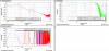
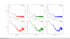
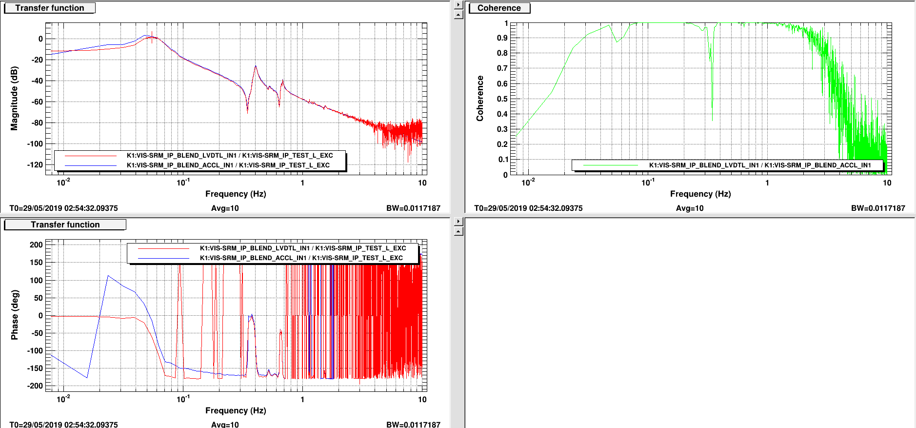
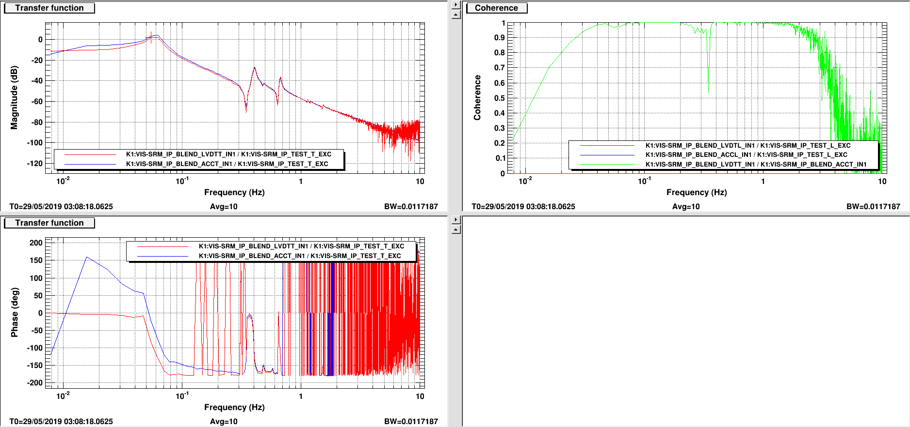
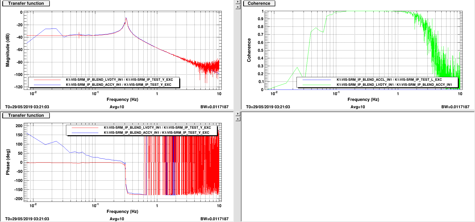
The coherence between LVDT signals and geophone signals ultimately determines the minimum frequency that we can choose to blend the two signals. After the diagonalization, I measured coherence between LVDT and geophones in terms of L, T and Y. See figure 2, 3, 4. From figure 2, 3, the coherence between LVDT and Geophone is ~1 above 50 mHz while in figure 4, the coherence is around 1 above 100 mHz. This means that we should blend L and T above 50 mHz and Y above 100 mHz. However, just to be safe, we limit the all blending frequencies to be above 100 mHz.
LVDT and Geophone Intrinsic Noise level
After consulting Okutomi-san and Fujii-san, I decided the fitting functions of the LVDT noise level and geophone noise level as follows:
LVDT: flat.
Geophone: From zero to resonance frequency: 1/f^3, the rest: flat.
I put the suspension into FLOAT state and measured the noise spectrum after it is sufficiently quiet. The noise spectrum and fitting curves can be seen in figure 5.
Blending Filter Optimization
The blending filter for IP in general composes of two filters, one being a "low pass" and the other being a "high pass", but has no definite functional form. LVDTs have lower noise compared to geophones at low frequencies. But, in higher frequencies, it is the other way around. Just because the problem is not complicated enough, the LVDTs are also coupled to the ground motion and therefore the LVDT noise is actually estimated to be the quadrature sum of the seismic noise and it's own noise. In particular, the seismic motion has a peak at around 200 mHz which we called the microseismic peak. This contributes to most of the rms motion of the optic as we discovered in 8918 where I studied the residual motion of the SR2. Therefore, we should take this into account and design the "low pass" filter such that the total noise is minimized. We can only design one filter because the other is automatically selected as 1 minus the other so that the blended signal has the same scale in all frequencies and is scaled to the same as the LVDTs and geophones signals. Lucia designed a generic blending LPF which is a combination of a 5th-order low pass, a 3rd-order low pass and three second-order zeros (reciprocal of a harmonic oscillaor). It has a 8th-order roll-off before 200 mHz to further decrease the contribution from the microseismic peak and returns to a 5th-order roll off at a slightly higher frequency. So, the bledning LPF is essentially a function that has 8 variables (2 cutoff frequencies, 3 resonance frequencies and 3 Q-factors).
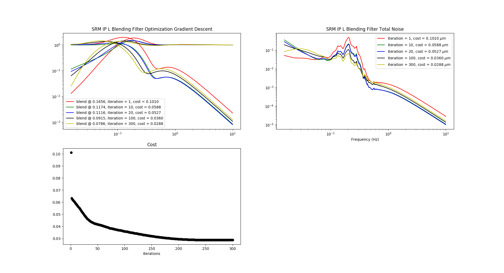
Previously, Lucia has been fine tuning those variables by hand adjustment so to minimize the total noise in the blended signal. However, I suspected that this fine tuning process can be done automatically by optimization algorithms. Therefore, I attempted to formulate the problem and use the widely used gradient descent method to try to look for an optimized blending filter. For a sanity check, I defined the cost function as the integrate RMS of the total noise and I begin optimizing the filter using Lucia's preivous blending filters with some random perturbation. Upon optimizing that filter for 10 iterations with a learning rate of 0.1, the total rms noise reduced from 0.101 µm to 0.0588 µm. But, the blending frequency was also reduced to 117.4 mHz which could be dangerous because the LVDTs and the geophones have weak coherence below 100 mHz. So, I terminated the process and manually adjusted the filter such that the noise level is further surpressed to 0.0578 µm but retaining the blending frequency. I installed those filters for IPL and IPT while using the old 260 mHz blending filter for IP Y. I measured TFs and confirmed that they did not deviate from the original TFs.
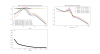
I copied the damping filters from the normal damping filters and pasted them to the inertial damping filter bank. And, I left the inertial damping on for the weekend to see if it is unstable. On Monday, everything is still intact. So, it shows preliminarily the possibility of automatic optimization of filters. The actual performance is yet to be confirmed and I intend to study the performance by looking at the optic's motion. For future use, I modified the optimization alogrithm to automatically decrease the learning rate when necessary to prevent from "over-learning" and then let it run for 1000 iterations. The result coverged at around 300 iterations, meaning that the best blending is found. See figure 6 for a shortlist of the filters' evolution and the corresponding noise levels. If possible, I would like to test the best filter in the future because it is simply perfect from the noise level suppression POV. At low frequency, it rolls off the high pass quickly to reduce geophone noise while having good performance in suppressing the microseismic peak at 200 mHz.
For future work, if time allows, I would like to define a more fancier cost function that also consider the coherence of the LVDTs and the geophones so the blending frequency is restricted.

