Last week we measured and implemented the sensing and driving matrix for the LVDTs and the actuators of ITMX Inverted pendulum (IP).
We give here some details of the measurements.
- Geometrical Sensing matrix: to correctly compute the sensing matrix it is essential to have informations about the exact arrangement of the sensors in the interferometer reference frame [X,Y]. We remind that the all LVDTs are distributed, in a plane geometry, on the vertices of an equilateral triangle (120 degrees between each to other and far from the center d = 594 mm) for this reason when the position of one of the LVDT is known it is possible derive the positions of other two from simple geometrical observations. For this purpose we have measured the position of the center of one of the LVDT (H1) and we found 6 degrees of difference with the nominal value (270 degrees). Moving in counter clokwise we found that the position of each sensors in the interferometer reference frame are:
- H1: a1=264 degree,
- H3 : a3=a1+120
- H2 : a2=a1+240.
By applying the standard geometrical transformations to these value we corrected the nominal sensing matrix.
Old matrix:
| H1 | H2 | H3 | |
| 0.666 | -0.333 | -0.333 | L |
| 0 | -0.5774 | 0.5774 | T |
| 0.5612 | 0.5612 | 0.5612 | Yaw |
New matrix:
| H1 | H2 | H3 | |
| -0.0697 | -0.5393 | 0.6090 | L |
| 0.6630 | -0.3918 | -0.2711 | T |
| 0.5612 | 0.5612 | 0.5612 |
Yaw |
In this way we have built up a set of virtual diagonalized LVDTs [L,T,Yaw] in the interferometer reference frame [X=L,T=Y and Yaw].
- Readout Driving matrix: To built the diagonalized virtual actuators we have chosen to measure the driving matrix referring at the readout of the diagonalized virtual sensors (L,T,Yaw). This measurement is done by injecting a line at with frequency f0 from each real actuator [Coil1, Coil2, Coil3] and by measuring module and phase of the transfer function between the j-th actuator and the diagonalized LVDTs [L ,T ,Yaw]. In this way it is possible to weigh the force (TF module) that each single real actuator must do to move only along the selected degree of freedom and the direction (TF phase). These numbers are stored for column in a matrix C whose the inverse is the driving matrix. A crucial point for the measurement of these matrices is the choice of the frequency f0. We reminde that these matrices have real coefficients: so it is important to choose a range in which the mechanical transfer function have give just real values (complex number whose phase is equal to zero, pi + 2n*pi). In the case of the inverted pendulum, it possible to choose or the DC region of the transfer function (TF is a constant value) or the region above the inner resonances of the system (where the TF goes like 1 / f ^ 2).
At low-frequency (few mHz) the measurement takes a long time (more or less 1 or 2 hours) to get a good resolution we opted for the region after the inner resonances (f0=3Hz); in fact the last resonance of the chain is expected at about 2 Hz, so at 3 Hz the behavior of the transfer function is 1 / f ^ 2.
Driving matrix:
| L | T | Yaw | |
| -0.6785 | -6.2277 | 1.82 | H1 |
| 4.3219 | -3.2813 | -1.085 | H2 |
| 4.9863 | 2.5122 | 1.3415 |
H3 |
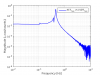
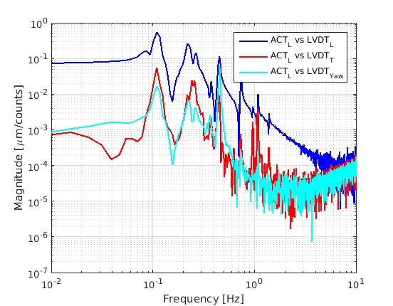
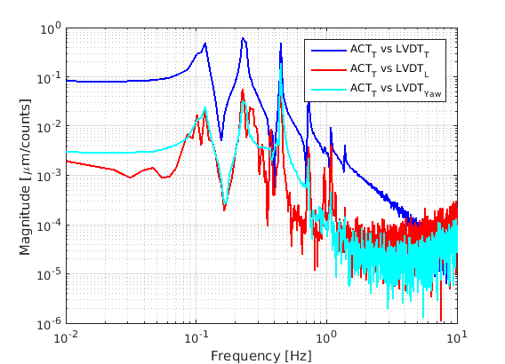
Attached to this report there are the measured transfer functions by injecting white noise from diagonalized virtual actuators and looking at diagonalized virtual LVDTs [Fig1,Fig2,Fig3]. We can observe that all degree of freedom are decoupled. We have evaluated the decoupling of the longitudinal degree of freedom (L) and Yaw: we found a factor 62 in the DC region and a factor 6 on the proper mode of IP Yaw motion (Fig1). At the same way we have estimated the decoupling of the transversal degree of freedom (T) with the Yaw: In this case we found a factor 28 in the DC region and a factor 3 on the proper mode of IP yaw motion (Fig2). In Fig3 we can see that the proper mode of Yaw is about 0.445 Hz.

